Instrument Alignment in SA Continued: Bundling & USMN
 In our previous newsletter article, we discussed methods in SpatialAnalyzer (SA) to align an instrument in order to compare measurements of an actual part to a nominal or ideal part. However, this only scratches the surface of SA’s alignment tools. Once you have more than one instrument station in a job, each new station must be aligned with every other station in order to create a network of measurements. SA provides three options for creating a network alignment: Best-Fit, Bundle Adjustment, and Unified Spatial Metrology Network (USMN).
Instrument Alignment in SA Continued: Bundling & USMN
In our previous newsletter article, we discussed methods in SpatialAnalyzer (SA) to align an instrument in order to compare measurements of an actual part to a nominal or ideal part. However, this only scratches the surface of SA’s alignment tools. Once you have more than one instrument station in a job, each new station must be aligned with every other station in order to create a network of measurements. SA provides three options for creating a network alignment:
- Best-Fit
- Bundle Adjustment
- Unified Spatial Metrology Network (USMN)
Best-Fit
Most measurement software packages provide a means to best-fit points together in order to align two instruments in 3D space. Accessed by a single right-click of an instrument, common points taken by the instrument can be fit to nominal design points or those taken from a previous instrument with complete control of every aspect of the fit. Degree of freedom constraints can be individually locked, individual points can be included or excluded, and weights can be modified to increase or decrease the influence of individual points, all while previewing the resulting fit. Once satisfied, the transformation can be applied to align the instruments (see Figure 1).
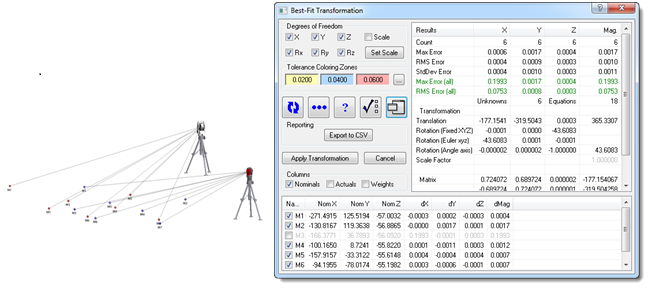
Figure 1: Best-Fit Transformation
Limitations of a Best-Fit Transformation for Network Alignment:
- Only two instruments can be fit together at a time. As a result, instrument stations must be chained together, one after another, causing error to rapidly propagate along the chain.
- No effective method exists to tie the ends of a chain together for better results, due to the fact that only two instruments are considered at a time.
- Best-fit does not provide a way to evaluate the quality of the network.
Bundle Adjustment
Two-D theodolites require a different treatment than best fit, so SA provides a bundle adjustment. In order to perform a bundle adjustment, each target shot is identified by a unique group and target name. Bundling seeks to minimize the amount that the shot rays from each instrument miss each other. Figure 2 shows an exaggerated case of missing a common target. With just one point, as shown, the rays can be made to exactly intersect. This is not the case when an entire network is solved. It becomes an optimization to minimize the discrepancies.
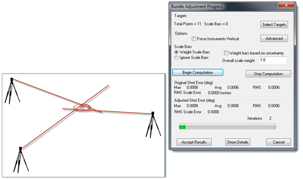
Figure 2: Bundling Instruments Together
Limitations of Bundling for Network Alignment:
- More targets are needed to bundle than the three required for a best-fit.
- Individual points are not weighted separately, preventing the individual characteristics of the instruments from being used in the alignment.
- In the case of trackers, bundling doesn’t automatically adjust weights for observation components.
Although bundling does present some limitations, it is a convenient alignment method and its use enables the incorporation of advanced theodolite network targeting such as collimation shots and mirror cubes.
Unified Spatial Metrology Network (USMN)
For situations in which the quality of alignment is critical, SA provides the ideal solution for network alignment. USMN is a bundling technique that optimizes instrument and target positions by intelligently using measurement uncertainty weighting. USMN provides a visual and measurable evaluation of the quality of an alignment, yielding three powerful benefits:
- USMN delivers an optimized set of points representing the most likely target positions, including a calculated uncertainty for each point.
- USMN provides a way to evaluate and determine the uncertainty in a specific instrument under real-world conditions including factors such as instrument uncertainty, tooling variation, operator performance, and environmental influence.
- USMN provides a way to obtain the best possible simultaneous network alignment solution, building upon the specific uncertainties of the instruments used in the network.
Understanding Instrument Uncertainty, the Foundation of USMN
“A measurement result is complete only when accompanied by a quantitative statement of its uncertainty.” –National Institute of Standards and Technology (NIST)
USMN was developed specifically to “fill in the gaps” of other network alignment methods. USMN provides an improved network solution, as well as calculates an uncertainty estimate based on the specific instruments that measured the points. To accomplish this, USMN does not merely consider the measured points in a network but also considers the statistical accuracy of those points by calculating an uncertainty cloud. This cloud defines the shape and size of a given measurement’s uncertainty field based on instrument characteristics. The characteristics of this cloud inherently depend on the accuracy of the instrument, the distance between the target and the instrument, and a number of other environmental and operational parameters. For instance, the greater the measurement distance, the larger and more diffuse the cloud (see Figure 3).
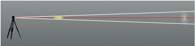
Figure 3: Changes in Cloud Shape with Distance
In addition, the vertical, horizontal, and distance components of the uncertainty for each instrument are considered independently. As a result, different instruments will have different cloud shapes for a particular point measurement. For example, a total station typically has better angular accuracy than distance accuracy. Alternatively, a tracker is extremely good at determining distance, but may not be as accurate as a total station in its angular measurements. The uncertainty clouds for these two types of instruments therefore have very different shapes. The total station with a greater uncertainty in distance will have a longer, thinner cloud whereas a tracker will have a more compact cloud that is wider due to its lower angular accuracy (see Figure 4).
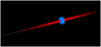
Figure 4: Comparison Between Point-Cloud Shapes Showing the Cloud from a Tracker
(Blue) and a Total Station (Red).
In order to mathematically calculate the cloud distributions, SA utilizes a Gaussian random number generator (utilizing a Box-Muller algorithm) because real-world, natural processes tend to have a Gaussian distribution. It builds uncertainty clouds in three dimensions based upon the uncertainty values of the instrument and the number of samples you specify for each point using a preset confidence interval (see Figure 5). The uncertainty values can be set independently for Theta, Phi, and distance for each instrument, although the default values are usually an excellent starting point.
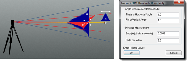
Figure 5: Instrument Uncertainty Values Can Be Set in the Properties of Each Instrument.
USMN Dialog How-to
Using USMN is deceptively simple for the amount of information and control available to the user. To begin, simply select the instruments you wish to include in the network alignment. SA then builds a list of common points shot by those instruments. When you open the USMN dialog, you will see three primary sets of data: the instrument list (which shows the instrument stations included in the network), the point target information (which shows the statistics for each point included in the fit), and the summary plane (which shows you the network solution summary) (see Figure 6).
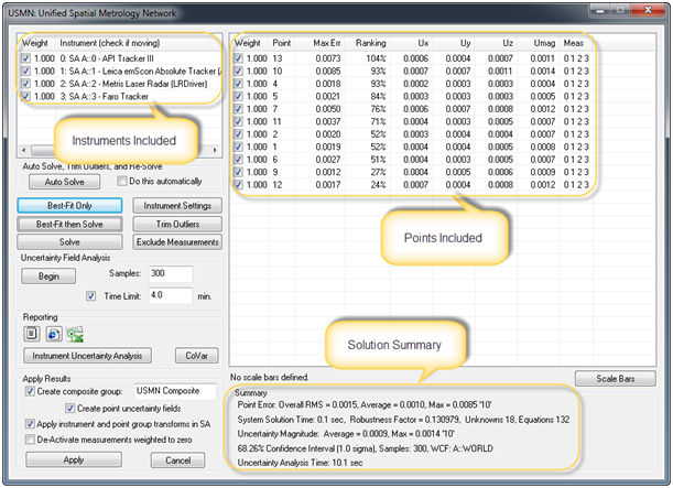
Figure 6: Primary USMN Dialog Information
Much like the best fit dialog, the initial values reported are the current instrument alignment conditions. By going to the Instrument Settings you can adjust the degrees of freedom of any instrument in the network, as well as the weighting individual instruments have on the overall fit (see Figure 7). Before you begin the fitting process, you may also want to use the Exclude Measurements button, which provides a filtered list of points that can be excluded from the network solution.
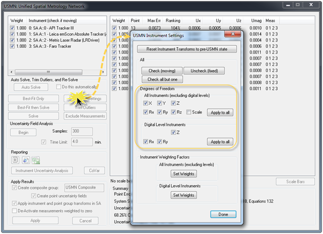
Figure 7: Instrument Settings in the USMN Dialog.
By clicking the Best-Fit Only button, the points are fit together using a pure best fit. While not absolutely necessary, this step provides a starting point or “initial condition” for the instruments, and generally leads to a faster solution. Clicking the Solve button then computes the actual USMN solution.
When looking at the statistics included for each point, you are given two primary pieces of information to evaluate: max error and ranking. From there, you can decide whether to include or exclude a point from the alignment. The max error for a point is the maximum distance between two measurements of a particular target (see Figure 8).
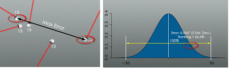
Figure 8: Max Error and Point Ranking Definitions.
Ranking is a quantitative indicator of measurement quality expressed as the percentage of the three sigma envelope the measurement residual is consuming. This ranking value is in many ways the best possible way of evaluating if either a point or a particular measurement of a point is an outlier and could be throwing off your fit. Any measurement with a ranking value greater than 100% is considered to be greater than three standard deviations from the mean and by definition falls outside of 99.74% of the data. Any point with this ranking or higher should be closely examined to determine if it is an outlier.
In addition to the point listing, you can also double-click on any particular point to get a listing of the same statistics for each individual measurement taken of a particular point (see Figure 9). This allows you to look at each measurement and decide if you wish to include or exclude the measurement, change its weighting, and evaluate its impact on the solution.
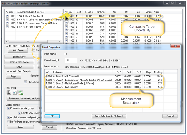
Figure 9: Double-click access to individual measurement statistics for a point.
A more efficient method is the Trim Outliers button, which will automatically go through and exclude points or measurements that are outside of a preset threshold, making it a single click to trim outliers.
Determining Instrument Uncertainty Values in a Network
In addition to calculating the uncertainty of a particular point based on a set of uncertainties for an instrument, SA also provides a means to turn that equation around and look at the uncertainties of a particular instrument. To be representative of real world accuracies, the best possible uncertainty values for a particular instrument under specific conditions should be used. These factors must include not only the instrument uncertainty, but also uncertainty introduced to the particular tooling, operator performance, and environmental conditions under which the measurements are being taken. SA provides a standard set of instrument accuracy settings which typically are quite good for normal situations. However, if you wish to see the performance of a particular instrument based upon the network solution, that information is a click away by performing an Instrument Uncertainty Analysis (see Figure 10).
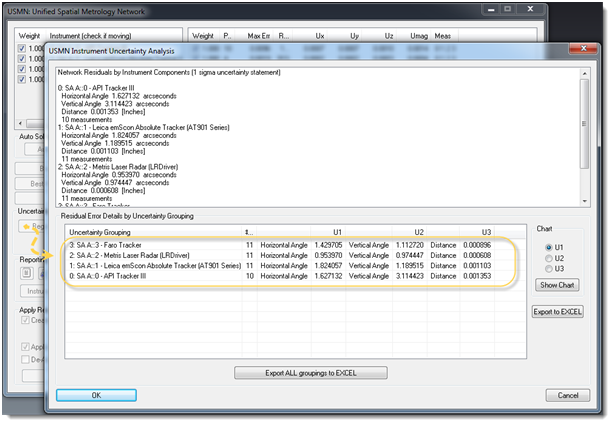
Figure 10: Instrument Uncertainty Values Resulting From an Instrument Uncertainty Analysis
Alternatively, if you wish to truly determine the best possible accuracy values for a particular instrument, you can set up a network of instrument stations measuring the same targets multiple times from different vantage points. This provides a means of evaluating the performance of your particular instrument under particular real-world conditions. Those values can then be used for the instrument uncertainties when you perform your true measurements and an even tighter network solution can be found.
Combining the tools to deliver the best possible network solution, evaluating not only the uncertainty of the points, measurements, and instruments for a given confidence interval, USMN provides a greatly improved network alignment solution for real world applications.
Questions? Contact NRK at support@kinematics.com.
Sign up to receive our eNewsletter and other product updates by clicking here.